Learning to Localize with TEM - Simple Spatial Agent

The key assertion that is examined by this project is that agents should learn a concept of space through their actions, and then use that space to remember and plan. The assertion is based in part on the function of the hippocampus in animal navigation, memory, and cognition. Whittington et al. published a model of the hippocampus called the Tolman Eichenbaum Machine with a later update using transformer attention for memory called TEM-t. I have discussed this method in detail on my blog. The approach in the current project is a variation of this scheme.

Our goal will be to develop a closed-loop, needs-driven controller on top of an auto-localization mechanism like TEM. By “auto-localization”, I mean localization through based strictly on the sensory input and action output, without any external observation of the explicit or true position. This concept is deeply akin to SLAM for robotics, and in fact, the approach here may be considered a form of neural SLAM.

Before working with a goal-driven controller, however, we will first develop the localization machinery and verify that it is working. We will do this by using a controller that traverses the space with random contents. During these traversals, we will train our localization models. Then we will inspect how the model has learned to represent space and make sure that this representation is acceptable.

Localization Problem Statement¶

Localization is to be based purely on sensor and actuator data. Thus we suppose that we have a sensor sequence $x = (x_1, x_2, \ldots, x_t, \ldots)$ and an action sequence $a = (a_1, a2, \ldots, a_t, \ldots)$ . We will use $x_{<t}$ for the sensor data up to but not including $x_t$ , and $x_{\leq t}$ for sensor data up to and including $x_t$ . The action $a_t$ is selected on the basis of $x_t$ and hence comes after $x_t$ .

We want to infer a latent sequence of locations $\ell = (\ell_1, \ell_2, ..., \ell_t, \ldots)$ such that $\ell_t$ represents the location in space where the agent observed $x_t$ and responded with action $a_t$ .

We will infer $\ell_t$ as a random variable in a probabilistic system, which means we will train a probability density $q_\phi$ defined so that

q_\phi(\ell \mid x, a) \,\,=\,\, \prod_t \,q_\phi\left(\ell_t \,\left\vert\,x_t,\,\vphantom{x^{x^x}} M(\ell_{<t},x_{<t}), \,a_{\leq t}, \,\ell_{t-1}\right.\right).

(1)

This model will be trained using a variation autoencoder (VAE), which means we will also train a reverse generative model $p_\theta$ as

p_\theta(x, \ell \mid a) \,\,=\,\, \prod_t \,p_\theta\left(x_t \,\left\vert\, \ell_t, \,M(\ell_{<t},x_{<t})\vphantom{x^{x^x}}\right.\right) \, p_\theta(\ell_t \mid \ell_{t-1}, \,a_t),

(2)

where the function $M(\ell_{<t}, x_{<t})$ in both models is a memory containing pairs of (location, sensory data) for all times preceding $t$ .

The component of the model that pertains to updating actions is $p_\theta(\ell_t \mid \ell_{t-1}, \,a_t)$ . For TEM-t in particular, the authors choose the inference model to be

\ell_t = \sigma(W_{a_t}\ell_{t-1})

(3)

for nonlinear activation function $\sigma$ (they use ReLU) and learned weight matrix $W_{a_t} = W(a_t)$ . From a theoretical standpoint, this is problematic because the outputs are forced to be non-negative, but the underlying distribution is assumed to be Gaussian, and hence supported across the reals. In practice, it may not matter, but this can be revisited.

As is normal for a VAE, we will train $p_\theta$ and $q_\phi$ to model the same distribution as closely as possible by maximizing the Evidence Lower Bound (ELBo),

\mathcal{L} \,\,=\,\, \mathbb{E}_{q_\phi}\left[\log \,\frac{p_\theta(x, \ell \mid a)}{q_\phi(\ell \mid x, a)}\right]

(4)

which, as usual, breaks down in two key terms after factoring the conditionals,

\mathcal{L} \,\,=\,\, \sum_t \left\{\vphantom{x^{x^{x^{x^{x^{x^x}}}}}}\mathbb{E}_{q_\phi}\left[\vphantom{x^{x^{x^{x^{x^x}}}}}\log p_\theta(x_t \mid\ldots)\right] \,\,-\,\, \mathrm{E}_{q_\phi}\left[\log \,\frac{q_\phi(\ell_t \mid \ldots)}{p_\theta\left(\ell_t \mid \ldots \right)}\right]\right\},

(5)

where the first term maximizes the probability of the training data under the generative model, and the second term is the Kullback-Leibler divergence of the generation model from the inference model:

\mathcal{L} \,\,=\,\, \sum_t \left\{\vphantom{x^{x^{x^{x^{x^{x^x}}}}}}\mathbb{E}_{q_\phi}\left[\vphantom{x^{x^{x^{x^{x^x}}}}}\log p_\theta(x_t \mid\ldots)\right] \,\,-\,\, D_{KL}\left({q_\phi(\ell_t \mid \ldots)} \,\left\|\, \vphantom{x^{x^{x^{x^{x^x}}}}}{p_\theta\left(\ell_t \mid \ldots \right)}\right.\right)\right\}.

(6)

The authors of the TEM paper present the model as a VAE, but their actual training seems to be a deterministic variation on the above, assuming standard normal distributions on each component, with sign reversed for minimization:

\mathcal{L}_{\text{det}} = \sum_t \left\{\vphantom{x^{x^{x^{x^{x^{x^x}}}}}}\mathbb{E}_{q_\phi}\left[ \frac{1}{2}\left\|\vphantom{x^{x^x}} x_t - \text{M.read}(\ell_t)\right\|^2 \,\,-\,\, \frac{1}{2}\left\|\vphantom{x^{x^x}} \ell_t - \text{M.sample}(x_t)\right\|^2 \,\,+\,\, \frac{1}{2}\left\|\vphantom{x^{x^x}} \ell_t - \sigma\left(W_{a_t} \ell_{t-1}\right)\right\|^2 \right] \right\}

(7)

where $\text{M.read}$ and $\text{M.sample}$ are memory reads (by key) and memory sample (by value). See Developing a Spatial Map for details. Note that

\ell_t = \frac{1}{2} \left(\vphantom{x^{x^x}}\sigma\left(W_{a_t} \ell_{t-1}\right) + \text{M.sample}(x_t)\right)

(8)

minimizes the difference in $\mathcal{L}_{\text{alt}}$ above.

Let’s make a diagram of the model to show the interactions:

from graphviz import Digraph

def tem_vae_timeslice():
    g = Digraph('G', format='svg')
    g.attr(rankdir='LR', splines='spline', nodesep='0.5', ranksep='0.6')
    node = lambda n, **kw: g.node(n, **({'shape':'ellipse', 'fontsize':'12'} | kw))

    # Styles
    obs = {'style':'filled', 'fillcolor':'#e8f0fe'}    # observed (x, a)
    lat = {'style':'filled', 'fillcolor':'#fff7e6'}    # latent (ℓ)
    det = {'shape':'box', 'style':'rounded,filled', 'fillcolor':'#eef7ee'}  # deterministic (M, factors)

    # Plates (clusters)
    with g.subgraph(name='cluster_tminus') as c:
        c.attr(label='t-1', color='#cccccc')
        c.node('l_tm1', 'ℓ_{t−1}', **lat)

    with g.subgraph(name='cluster_t') as c:
        c.attr(label='t', color='#cccccc')
        c.node('x_t', 'x_t', **obs)
        c.node('a_t', 'a_t', **obs)
        c.node('l_t', 'ℓ_t', **lat)
        c.node('M_t', 'M(ℓ_{<t}, x_{<t})', **det)

    with g.subgraph(name='cluster_tplus') as c:
        c.attr(label='t+1', color='#cccccc')
        c.node('l_tp1', 'ℓ_{t+1}', **lat)

    # Generative edges pθ:
    g.edge('l_t', 'x_t', label='pθ(x_t | ℓ_t, M)', fontsize='10')
    g.edge('M_t', 'x_t', color='#5b8', fontsize='10')
    g.edge('l_tm1', 'l_t', label='pθ(ℓ_t | ℓ_{t−1}, a_t)', fontsize='10')
    g.edge('a_t', 'l_t', color='#5b8')

    # Inference info qφ (dashed helpers into ℓ_t)
    g.edge('x_t', 'l_t', style='dashed', color='#888', label='qφ', fontsize='10')
    g.edge('M_t', 'l_t', style='dashed', color='#888')
    g.edge('l_tm1', 'l_t', style='dashed', color='#888')

    # Temporal link forward (light)
    g.edge('l_t', 'l_tp1', style='invis')  # keep layout tidy

    return g

tem_vae_timeslice()

Upgrading TEM’s Spatial Content¶

Now we will develop the variant of the TEM model in tree_world.models.tem. This is not strictly either TEM or TEM-t, because it uses the memory described in Developing a Spatial Map instead of a Hopfield net or a standard transformer layer. But it is the same model in spirit.

We begin with a component for updating localization based on action. As noted above, TEM-t uses $\ell_t = \sigma(W_{a_t}\ell_{t-1})$ . But this assumes discrete actions (e.g., north, south, east, west) with one distinct matrix $W_a$ per action. Furthermore, the grid sizes explored in the TEM paper are quite small, 11x11 at the largest. We will work with continuous actions in larger spaces, so we will need to think more deeply about what $\ell_t$ represents and what $W_a$ is intended to do.

The purpose of TEM is to model the grid cells of the entorhinal cortex. Grid cells fire in a sort of Fourier representation of the position. For now, we will avoid the fourier representation in favor of a model where a neuron fires when the agent is at a particular spot in its internal map. This means that $\ell_t$ should be a sparse vector of high dimension, and could be organized either as a vector (for 1-D maps) or a matrix (for 2-D maps), or even as a 3-tensor (for 3-D). We should assume that actions are local, transferring activity among neighboring grid cells but leaving distant grid cells untouched. Yet we should also want our actions to be translation invariant, applying action equally at various points in space. These two considerations point towards an implementation with a convolutional layer over a pixel-like space.

Note that we can later implement a Fourier transformation of the pixel-like space to obtain a more biologically faithful model.

To represent the space of tree world in this pixelated way, consider a spatial grid of size $S \times S$ for integer $S > 0$ , that is, let $\ell \in \mathbb{R}^{S\times S} \approxeq \mathbb{R}^{S^2}$ , and suppose $S = 2R + 1$ for another integer $R$ , so that the bounds of the space are $[-R, R]$ in each dimension. Let us assume a spatial scale $\gamma > 0$ , and let us interpret $\ell_{ij}$ to represent the point $\left(\vphantom{x^{x^x}}\gamma (i - R), \gamma (j-R)\right)$ in $\mathbb{R}^2$ .

Under this interpretation, $\ell$ becomes a probability distribution over $\mathbb{R}^2$ representing the agent’s belief about its location in $\mathbb{R}^2$ .

For our basic actions in Tree World, we have $a_t \in \mathbb{R}^2$ performing a translation in the underlying space. While we might want more complicated actions later, this choice makes our modeling straightforward for now. First, we can define a continuous 2-D convolution kernel

\hat{W}[a](h,w) = \left\{\begin{array}{cc} 1 & \text{if $a = (-w,-h)$} \\ 0 & \text{otherwise} \end{array}\right.,

(9)

which, when convolved with a location belief map, will translate the location beliefs according to the vector $a$ .

Now we need to replace $\hat{W}[a]$ into a discrete kernel of size $S \times S$ . Rather than write down the math, let’s just give the code:

import torch
import torchvision


def map_index_to_space(indices, R, gamma):
    return gamma * (indices - R)

def map_space_to_preindex(x, R, gamma):
    return x / gamma + R

def make_2d_translation_kernel(a, gamma=1.0, filter_size=5, 
                               apply_gaussian_blur=False, gaussian_blur_kernel_size=3, gaussian_blur_sigma=1):
    """
    Make a discrete translation kernel for action a in a space of size S.
    """
    if a.ndim == 1:
        a = a.unsqueeze(0)

    assert a.ndim == 2
    assert a.shape[1] == 2
    assert filter_size % 2 == 1, "filter_size must be odd so that the center is well-defined"

    channels = a.shape[0]
    K = (filter_size - 1) // 2

    # note: we negate a here because we want to translate in the direction of a -- positive would move the opposite direction
    actual = map_space_to_preindex(-a, K, gamma)
    upper = torch.ceil(actual)
    lower = torch.floor(actual)
    fraction = (actual - lower) / (upper - lower)
    fraction_mask = (upper - lower) < 1e-8
    fraction = torch.where(fraction_mask, torch.ones_like(fraction), fraction)

    # note: we reverse the indices because typical image indexing is (y, x) but our actions are (x, y)
    outer_indices = torch.arange(channels)
    upper_indices = torch.clamp(upper.long(), 0, filter_size - 1)
    lower_indices = torch.clamp(lower.long(), 0, filter_size - 1)

    action_filter = torch.zeros(channels, channels, filter_size, filter_size)
    
    fraction_x = fraction[..., 0]
    fraction_y = fraction[..., 1]

    fraction_x_opp = torch.where(fraction_mask[..., 0], torch.ones_like(fraction_x), 1 - fraction_x)
    fraction_y_opp = torch.where(fraction_mask[..., 1], torch.ones_like(fraction_y), 1 - fraction_y)

    action_filter[outer_indices, outer_indices, upper_indices[..., 1], upper_indices[..., 0]] = fraction_y * fraction_x
    action_filter[outer_indices, outer_indices, lower_indices[..., 1], lower_indices[..., 0]] = fraction_y_opp * fraction_x_opp
    action_filter[outer_indices, outer_indices, upper_indices[..., 1], lower_indices[..., 0]] = fraction_y * fraction_x_opp
    action_filter[outer_indices, outer_indices, lower_indices[..., 1], upper_indices[..., 0]] = fraction_y_opp * fraction_x

    if apply_gaussian_blur:
        import torchvision
        kernel_size = [gaussian_blur_kernel_size] * 2
        gaussian_sigma = [gaussian_blur_sigma] * 2
        action_filter = torchvision.transforms.functional.gaussian_blur(action_filter, kernel_size, gaussian_sigma)

    return action_filter


print(f"action [1, 1]")
action_filter = make_2d_translation_kernel(torch.tensor([1, 1]))
for row in action_filter.squeeze():
    print(" ".join(f"{x:.2f}" for x in row))

print()
print(f"batch size 2, actions [[1, 0], [-0.4, -0.25]]")
action_filter = make_2d_translation_kernel(torch.tensor([[1, 0], [-0.4, -0.25]]))
print("------[1, 0]------")
for row in action_filter[0,0]:
    print(" ".join(f"{x:.2f}" for x in row))

print()
print(f"Check zeros: {torch.norm(action_filter[0, 1, :, :])} = 0.0")
print()
print("------[-0.5, -0.5]------")
for row in action_filter[1,0]:
    print(" ".join(f"{x:.2f}" for x in row))

print()
print(f"Check zeros: {torch.norm(action_filter[1, 0, :, :])} = 0.0")

action [1, 1]
0.00 0.00 0.00 0.00 0.00
0.00 1.00 0.00 0.00 0.00
0.00 0.00 0.00 0.00 0.00
0.00 0.00 0.00 0.00 0.00
0.00 0.00 0.00 0.00 0.00

batch size 2, actions [[1, 0], [-0.4, -0.25]]
------[1, 0]------
0.00 0.00 0.00 0.00 0.00
0.00 0.00 0.00 0.00 0.00
0.00 1.00 0.00 0.00 0.00
0.00 0.00 0.00 0.00 0.00
0.00 0.00 0.00 0.00 0.00

Check zeros: 0.0 = 0.0

------[-0.5, -0.5]------
0.00 0.00 0.00 0.00 0.00
0.00 0.00 0.00 0.00 0.00
0.00 0.00 0.00 0.00 0.00
0.00 0.00 0.00 0.00 0.00
0.00 0.00 0.00 0.00 0.00

Check zeros: 0.0 = 0.0

def apply_2d_translation(
    location_belief, action, gamma=1.0, filter_size=5, 
    apply_gaussian_blur=False, gaussian_blur_kernel_size=5, gaussian_blur_sigma=2
):
    # location belief is a tensor of shape (batch_size, height, width)
    kernel = make_2d_translation_kernel(
        action, 
        gamma=gamma, 
        filter_size=filter_size, 
        apply_gaussian_blur=apply_gaussian_blur, 
        gaussian_blur_kernel_size=gaussian_blur_kernel_size,
        gaussian_blur_sigma=gaussian_blur_sigma
    )
    convolved = torch.nn.functional.conv2d(location_belief, kernel, padding=(kernel.shape[2] // 2, kernel.shape[3] // 2))
    return convolved

grid_size = 101   # R = 50
grid_points = torch.linspace(-1, 1, grid_size)
grid = torch.cartesian_prod(grid_points, grid_points).view(grid_size, grid_size, 2)  # (101, 101, 2), [-1, 1]^2
print(f"grid.shape: {grid.shape}")

gauss_img = torch.exp(-grid.pow(2).sum(dim=-1))
print(f"gauss_img.shape: {gauss_img.shape}")
shifted_gauss_img = apply_2d_translation(gauss_img.unsqueeze(0), torch.tensor([10, 10]), filter_size=31).squeeze(0)

# combine the images, initial on the left, translated on the right -- flip the height dim so that 0,0 is in the bottom left
matplotlib_img = torch.cat([gauss_img, shifted_gauss_img], dim=1).flip(dims=(0,))

from matplotlib import pyplot as plt

plt.imshow(matplotlib_img)

grid.shape: torch.Size([101, 101, 2])
gauss_img.shape: torch.Size([101, 101])

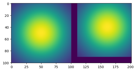
As the example above shows, the function make_2d_translation_kernel will output a kernel with shape (batch_size, batch_size, filter_height, filter_width) that can be applied as a 2d convolution to an image of size (batch_size, height, width) in channel_first format, and, when appropriately padded, will produce the same shape output, translated by action $a$ . In the example above, we move the image by 10 steps up and to the right in a space that has $S=200$ width.

We can also shift a batch size of two images with different actions. Below, we shift the top row 10 to the right, and the bottom row 10 down and 3 to the left.

# now shift two images at once
action = torch.tensor([[10, 0], [-3, -10]])
images = gauss_img.unsqueeze(0).repeat(2, 1, 1)
shifted_images = apply_2d_translation(images, action, filter_size=31)

matplotlib_img = torch.cat([
    torch.cat([images[0], shifted_images[0]], dim=1).flip(dims=(0,)),
    torch.cat([images[1], shifted_images[1]], dim=1).flip(dims=(0,))
], dim=0)

plt.imshow(matplotlib_img)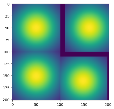

With apply_2d_translation, we can apply a movement action $a$ to a belief about locations $\ell$ . Let us call this translation $h$ and represent our new location as

\ell_t = h(\ell_{t-1}, a_t) \quad\quad\text{in place of}\quad\quad \ell_t = \sigma(W_{a_t} \ell_{t-1}) \quad\quad\text{above}

(10)

Note that the Fourier tranform of the convolution in $h$ will be a multiplication like $W_{a_t} \ell_{t-1}$ , so that our model is in agreement with the TEM model.

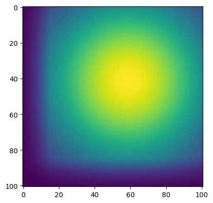
We can also use a gaussian blur to account for uncertainty in our action measurements, shown below.

shifted_gauss_img = apply_2d_translation(
    gauss_img.unsqueeze(0), torch.tensor([10, 10]), filter_size=31,
    apply_gaussian_blur=True, gaussian_blur_kernel_size=25, gaussian_blur_sigma=10
).squeeze(0)

plt.imshow(shifted_gauss_img.flip(dims=(0,)))

Revising the Memory for Location Beliefs¶

In Developing a Spatial Map, we developed a map keyed by locations. However, the keys were explicitly points in the location space, whereas our location beliefs $\ell_t$ is a grid of fixed locations. So, in Mapping Space With Location Beliefs, we developed a spatial map based on discretized grids. We will use the latter for our TEM variant. We need to understand the memory cost.

Our grid has size $S \times S$ . With a batch size of $B$ and a sensory dimension of $D$ , our storage requirement for $T$ timesteps of memory is $BTS^2$ for the locations and $BTD$ for the sensory data, or $BT(S^2 + D)$ for the whole. Now suppose we are willing to allocate 1GB to each member of the batch with FP8 precision; then we require

\log_2 \left|TS^2 + TD\right| \,\,=\,\, \log_2 T + \log_2\left| S^2 + D\right|\,\,\leq\,\, 30

(11)

If we set $T = 2^{15} = 32,768$ , $S < 2^7$ and $D = 1024 = 2^{10}$ , then we will be well under our budget. With $S = 101$ , we can even fit FP16 precision within 16GB. At 10 frames per second, we can fit almost an hour of time into our context (10 fps x 60s x 60m = 36,000 frames). With pruning we can reduce this requirement further. As a consequence, storage capacity does not limit our options.

What does limit us is the ability to read and sample the memory at 10 frames per second. So how fast can the memory run, and what kind of hardware will we need?

Implementing a TEM Module¶

We can use a single model to implement TEM as a pseudo-VAE; there is no good reason to maintain the inspiration of an encoder and decoder model. Instead, we need to build a module to infer $\ell_t$ , populate a memory $M$ , and compute the loss

\mathcal{L}_{\text{det}} = \sum_t \left\{\vphantom{x^{x^{x^{x^{x^{x^x}}}}}}\mathbb{E}_{q_\phi}\left[ \frac{1}{2}\left\|\vphantom{x^{x^x}} x_t - \text{M.read}(\ell_t)\right\|^2 \,\,-\,\, \frac{1}{2}\left\|\vphantom{x^{x^x}} \ell_t - \text{M.sample}(x_t)\right\|^2 \,\,+\,\, \frac{1}{2}\left\|\vphantom{x^{x^x}} \ell_t - h(\ell_{t-1}, a_t)\right\|^2 \right] \right\}

(12)

If we adopt the value

\ell_t = \frac{1}{2} \left[\vphantom{x^{x^x}}h(\ell_{t-1}, a_t) + \text{M.sample}(x_t)\right],

(13)

this reduces to

\mathcal{L}_{\text{det}} = \frac{1}{2}\sum_t \left\{\vphantom{x^{x^{x^{x^{x^{x^x}}}}}}\mathbb{E}_{q_\phi}\left[ \left\|\vphantom{x^{x^x}} x_t - \text{M.read}(\ell_t)\right\|^2 \right] \right\}

(14)

which will be minimized when the memory contains the right sensory data ( $\text{M.read}(\ell_t) = x_t$ ) at the location determined by checking the memory ( $\text{M.sample}(x_t)$ ) and predicting from the last position ( $h(\ell_{t-1}, a_t)$ ).

In practice, however, there are certain pathologies from always setting $\ell_t$ to the midpoint. Principally, at t=2, the memory only has the value from t=1, and this is what it will sample. This will pull $\ell_t$ towards its initial position, and the movement will never pick up. So instead, we choose the estimator

\ell_t = \frac{1}{2} \left[\vphantom{x^{x^x}}h(\ell_{t-1}, a_t)\times (1+s_t^\alpha) + \text{M.sample}(x_t)\times (1 - s_t^\alpha)\right],

(15)

for $\alpha > 1$ (e.g., $\alpha=10$ ) and

s_t \propto \left(\vphantom{x^{x^x}}\text{M.read}(\ell_{t-1}) \cdot \text{M.read}\left(\text{M.sample}(x_t)\right)\right)_+,

(16)

with inputs normalized to unit vectors, which is in $[0,1]$ and will be close to 1 if the sampled value reads the same sensory data as the last location belief. In essence, the factor $(1\pm s_t^\alpha)$ says that if the memory’s estimation of sensor reads haven’t changed, then trust the movement model, not the memory. A high $\alpha$ value is intended to favor use of the memory. This assumption means that the loss must include all three terms.

With this in mind, and using the memory as a parameter, we can implement TEM as follows.

import math
from tree_world.models.memory_belief import LocationBeliefMemory, create_initial_gaussian_belief

class TEM2d(torch.nn.Module):
    def __init__(self, 
        grid_size: int, sensory_dim: int, embed_dim: int, batch_size: int = 1, 
        grid_extent: float = 1000.0, max_action_norm: float = 5.0, use_memory_to_localize: bool = True
    ):
        super().__init__()
        self.batch_size = batch_size
        self.grid_size = grid_size        # S
        self.grid_extent = grid_extent    # how far across on each side, in "real world" units
        self.grid_scale = grid_extent / (grid_size - 1)  # gamma
        self.action_filter_size = 2 * int(math.ceil(max_action_norm)) + 1
        self.max_action_norm = max_action_norm
        self.use_memory_to_localize = use_memory_to_localize
        
        # create the memory
        location_dim = 2
        self.memory = LocationBeliefMemory(
            location_dim,
            sensory_dim,
            embed_dim,
            batch_size=batch_size,
            max_memory_size=grid_size**2,
        )
        
        self.sharpen_factor = 1.05
    
    def reset(self):
        self.memory.reset()
    
    def break_training_graph(self):
        self.memory.break_training_graph()

    def forward(self, last_location_belief: torch.Tensor, action: torch.Tensor, sensory_input: torch.Tensor,
                affinity_exponent: float = 20.0):
        if last_location_belief is None:
            # make a gaussian map centered at the origin
            last_location_belief = create_initial_gaussian_belief(self.grid_size // 2, self.grid_scale) # sd=0.25*self.max_action_norm)

        if torch.norm(action) > self.max_action_norm:
            print(f"WARNING: Action norm {torch.norm(action)} is greater than max action norm {self.max_action_norm}; action predictor will have errors")

        N, S, _ = last_location_belief.shape

        # estimate the new location belief
        inferred_location_belief = apply_2d_translation(
            last_location_belief,
            action,
            gamma=self.grid_scale,
            filter_size=self.action_filter_size,
        )

        if self.use_memory_to_localize:
            sampled_location_belief = self.memory.sample(
                sensory_input, 
                reference_location=last_location_belief, 
                reference_match_threshold=0.01,
                num_samples=25,
                aggregate=True
            )
            
            if sampled_location_belief is None or torch.norm(sampled_location_belief) < 1e-6:
                location_belief = inferred_location_belief
            else:
                location_belief = (sampled_location_belief + inferred_location_belief) / 2
        
        else:
            location_belief = inferred_location_belief

        # sharpen, since convolution blurs
        if self.sharpen_factor != 1.0:
            location_belief = location_belief.pow(self.sharpen_factor)

        # additional ... makes no difference to the math, but turns location_belief into a probability distribution
        location_belief = (
            location_belief / location_belief.view(location_belief.shape[0], -1).sum(dim=-1).view(N, 1, 1)
        )

        # estimate the sensory input from the location belief
        estimated_sensory_input = self.memory.read(location_belief)

        # compute the loss
        loss = (sensory_input - estimated_sensory_input).pow(2).mean()
        if self.use_memory_to_localize and sampled_location_belief is not None:
            loss = (
                loss
                + (location_belief - inferred_location_belief).pow(2).mean()
                + (location_belief - sampled_location_belief.squeeze(1)).pow(2).mean()
            )

        # update the memory
        self.memory.write(location_belief, sensory_input)

        return location_belief, loss

    @classmethod
    def from_config(cls, config: 'TreeWorldConfig'):
        return cls(
            config.grid_size, 
            config.sensory_embedding_dim, 
            config.dim, 
            1, 
            config.grid_extent, 
            max_action_norm=config.max_action_norm,
            use_memory_to_localize=config.use_memory_to_localize
        )

At present, our TEM model has zero parameters. Later on, we might want to add parameters

to compress location beliefs and sensory data prior to storing
to learn the affects of actions that implement movement implicitly

However, for testing purpose, TEM2d can be used immediately without training.

Adding an Agent Model¶

Our first experiment for TEM2d will use an agent model that deterministically spirals out from the origin.

from tree_world.simulation import AgentModel
from typing import Optional


class PathTracingTEM2dAgent(AgentModel):
    def __init__(
        self, 
        tem_model: TEM2d=None,
        time_to_rotate_spiral: int=100,
        time_to_rotate_heading: int=25,
        distance_increment_first_spiral: float=25,
        action_noise: Optional[float]=None
    ):
        self.t = 0

        self.alpha = distance_increment_first_spiral / time_to_rotate_spiral
        self.beta = 2 * math.pi / time_to_rotate_spiral
        self.gamma = 2 * math.pi / time_to_rotate_heading

        self.sign = 1.0

        self.tem = tem_model
        self.last_location = None
        self.last_action = None

        self.location_history = []
        self.actual_location_history = []

        self.loss = []

        self.action_noise = action_noise
        self.action_norm = 0.0

        self.optimizer = torch.optim.Adam(self.tem.parameters(), lr=1e-3)

    def reset(self):
        self.tem.reset()
        self.t = 0
        self.location_history = []
        self.actual_location_history = []
        self.loss = []

        self.last_location = None
        self.last_action = None
        
    def coords(self, t):
        r = self.alpha * t
        th = self.beta * t

        return torch.tensor([r * math.cos(th), r * math.sin(th)])

    def get_action(self, distance: float, embedding: torch.Tensor, heading: torch.Tensor, health: float,
                   agent_location: torch.Tensor=None, obj_location: torch.Tensor=None):

        if self.last_action is None:
            self.last_action = torch.zeros(1, 2)

        if self.action_noise is not None:
            self.last_action = self.last_action + torch.randn_like(self.last_action) * self.action_noise

        location_belief, loss = self.tem(self.last_location, self.last_action, embedding[None, :])
        self.last_location = location_belief
        self.location_history.append(location_belief)
        self.actual_location_history.append(agent_location)
        self.loss.append(loss)

        ph = self.gamma * self.t

        start_coords = self.coords(self.t)
        end_coords = self.coords(self.t + 1)
        position_delta = end_coords - start_coords

        new_heading = torch.tensor([math.cos(ph), math.sin(ph)])
        self.last_action = position_delta[None, :]

        self.t = self.t + 1
        self.action_norm = torch.norm(position_delta) * (1 / self.t) + self.action_norm * (self.t - 1) / self.t

        return position_delta, new_heading

    def train(self):
        print(f"Taking an optimizer step with {len(self.loss)} loss values")
        self.optimizer.zero_grad()
        torch.stack(self.loss).sum().backward()
        self.optimizer.step()
        self.loss = []
        self.tem.break_training_graph()
    
    @classmethod
    def from_config(cls, config: 'TreeWorldConfig'):
        tem_model = TEM2d.from_config(config)
        return cls(tem_model, action_noise=config.action_noise)

Running a Simulation¶

With an agent model, we can run our simulation.

S = 101   # grid size
D = 1024  # sensory dimension

from tree_world.simulation import TreeWorldConfig, TreeWorld, SimpleSensor
config = TreeWorldConfig()
config.embedding_dim = D
config.grid_size = S
config.model_type = "PathTracingTEM2dAgent"
config.num_trees = 50
config.action_noise = None
config.max_action_norm = 20.0
config.use_memory_to_localize = True
sensor = SimpleSensor.from_config(config)
world = TreeWorld.random_from_config(config)

We’ll run a simulation with the TEM2d model, capturing the locations and location beliefs along the way. For this simulation, we won’t allow the organism to die, so that we can map the whole space.

steps = 1000

print(f"Running tree world for {steps} steps...")
world.run(steps, record=True, allow_death=False)
print()
print("Tree world run complete.")

print(f"Agent health: {world.agent.health}")
print(f"Agent fruit eaten: {world.agent.fruit_eaten}")
print(f"Agent poisonous fruit eaten: {world.agent.poisonous_fruit_eaten}")
print(f"Agent total movement: {world.agent.total_movement}")
print(f"Agent final location: {torch.norm(world.agent.location).item()}")

Running tree world for 1000 steps...
Taking an optimizer step with 101 loss values
Taking an optimizer step with 100 loss values
Taking an optimizer step with 100 loss values
Taking an optimizer step with 100 loss values
Taking an optimizer step with 100 loss values
Taking an optimizer step with 100 loss values
Taking an optimizer step with 100 loss values
Taking an optimizer step with 100 loss values
Taking an optimizer step with 100 loss values

Tree world run complete.
Agent health: -72.65829467773438
Agent fruit eaten: 44
Agent poisonous fruit eaten: 12
Agent total movement: 7863.29345703125
Agent final location: 250.0

location_belief_history = torch.cat(world.agent.model.location_history, dim=0)
actual_location_history = torch.stack(world.agent.model.actual_location_history)
losses = torch.stack(world.agent.model.loss)

print(location_belief_history.shape)
print(actual_location_history.shape)

print(losses.shape)
print(f"Loss min: {losses.min()}, mean: {losses.mean()}, max: {losses.max()}")

torch.Size([1000, 101, 101])
torch.Size([1000, 2])
torch.Size([99])
Loss min: 7.400276081170887e-05, mean: 0.020602785050868988, max: 0.08758453279733658

Note that our affinities range from about 80% to 100% with an average around 95%. That means the memory sample is not being used much to choose the next location, but this is partly because this agent is constantly in a regime of exploring new space. We’ll try some more repetitive trajectories below.

Ok, let’s make a little video of how the location belief evolves over time, noting that

The location belief is initialized around the origin
The actions are known exactly and correctly

import matplotlib.pyplot as plt
from matplotlib.animation import FuncAnimation
from IPython.display import HTML
import torch
import matplotlib
matplotlib.rcParams['animation.embed_limit'] = 2**28


def display_location_belief_history(location_belief_history, actual_location_history):
# assume these are already defined:
# location_belief_history: (T, 101, 101)
# actual_location_history: (T, 2)
    T, H, W = location_belief_history.shape

    # Get min/max once so color scale doesn't jump
    vmin = float(location_belief_history.min())
    vmax = float(location_belief_history.max())

    extent = [-500, 500, -500, 500]  # [x_min, x_max, y_min, y_max]

    fig, ax = plt.subplots(figsize=(6, 6))

    im = ax.imshow(
        location_belief_history[0],
        extent=extent,
        origin='lower',          # y increases bottom→top
        vmin=vmin,
        vmax=vmax,
        cmap='viridis',
        interpolation='nearest',
    )
    agent_dot, = ax.plot(
        actual_location_history[0, 0].item(),
        actual_location_history[0, 1].item(),
        marker='o',
        color='red',
        markersize=6,
    )

    for tree in world.trees:
        x, y = tree.location.cpu().numpy()
        color = "red" if tree.is_poisonous else "green"
        ax.scatter(
            y, x,
            c=color, marker="x" if tree.is_poisonous else "o",
            s=80, edgecolor="k"
        )

    ax.set_xlabel("x")
    ax.set_ylabel("y")
    ax.set_title("Location belief over time")
    plt.close(fig)  # prevent duplicate static display in Jupyter

    def update(frame):
        # update heatmap
        im.set_data(location_belief_history[frame])

        # update agent dot
        x, y = actual_location_history[frame].tolist()
        agent_dot.set_data([x], [y])

        ax.set_title(f"Location belief – t={frame}")
        return im, agent_dot

    anim = FuncAnimation(
        fig,
        update,
        frames=range(0, T, 4),       # or range(0, T, step) to subsample
        interval=50,    # milliseconds per frame
        blit=True,
    )

    return anim

anim = display_location_belief_history(location_belief_history, actual_location_history)
HTML(anim.to_jshtml())

/var/folders/gw/zsqsy8v12h1fsqw6ph5ndprc0000gn/T/ipykernel_51820/4065992388.py:43: UserWarning: You passed a edgecolor/edgecolors ('k') for an unfilled marker ('x').  Matplotlib is ignoring the edgecolor in favor of the facecolor.  This behavior may change in the future.
  ax.scatter(

What went wrong?¶

In the plot above, the location belief does not move from the origin. Why not? Well, we incorporate $\text{M.sample}(x_t \mid \ell_{t-1})$ $into our estimator for$ \ell_t $. But$ \ell_t = W_{a_t} \star \ell_{t-1} $was already correct, since the action is perfectly known, and hence this extra estimator can only make$ \ell_t $worse. In fact, we are using the memory$ M$ that is populate only with the information seen before, and we are visiting unseen locations. So the memory contents are worthless for predicting the new sensory information. If the new sensory information changes to slowly, the memory will always just provide the last location as its guess for the agent’s current location. Worse, it will then write the new, slowly changing sensory information into the memory at the same location, asserting and reinforcing that the agent has not moved. In consequence, the location estimate will not move until the agent has gotten to a point where the input has changed too much, and the memmory can no longer produce any estimate. This is what we observe in the plot above.

For TEM, the authors used small discreate location spaces, where the observation would often visit the same location in a small graph. This has two different effects:

each action produces materially distinct sensory information
the same spot is routinely visited multiple times

Neither of these conditions is available to us in our continuous spaces.

In our setting, using a memory to predict location is only beneficial for two cases

Initial localization for reentering a previously explored space with a known map
Ongoing error correction if our action model is subject to systematic error or noise

But if we can’t use the memory to localize, then we do not need the VAE at all; we merely wish to minimize

\mathcal{L}_{\text{simple}} = - \sum_t \mathbb{E}\left[p_\theta(x_t \mid \ell_t)\right]

(17)

subject to $\ell_t = h(\ell_{t-1}, a_t)$ . Of course, in the zero-parameter version it makes no difference, but we do intend to add parameters.

In particular, a memory is useless for predicting location unless the sensor variation is of sufficient scale to detect differences at the scale of the per-step movement. And it isn’t even enough just to set the variance of the initial location belief to be small (tried it), because the sensor change at one step is small, so that the localizer still falls into this trap.

Let’s see the effect if we leave out the memory when predicting the location.

world.agent.model.tem.use_memory_to_localize = False

steps = 1000

print(f"Running tree world for {steps} steps...")
world.run(steps, record=True, allow_death=False)
print()
print("Tree world run complete.")

print(f"Agent health: {world.agent.health}")
print(f"Agent fruit eaten: {world.agent.fruit_eaten}")
print(f"Agent poisonous fruit eaten: {world.agent.poisonous_fruit_eaten}")
print(f"Agent total movement: {world.agent.total_movement}")
print(f"Agent final location: {torch.norm(world.agent.location).item()}")
location_belief_history = torch.cat(world.agent.model.location_history, dim=0)
actual_location_history = torch.stack(world.agent.model.actual_location_history)
losses = torch.stack(world.agent.model.loss)

print(location_belief_history.shape)
print(actual_location_history.shape)

Running tree world for 1000 steps...
Taking an optimizer step with 101 loss values
Taking an optimizer step with 100 loss values
Taking an optimizer step with 100 loss values
Taking an optimizer step with 100 loss values
Taking an optimizer step with 100 loss values
Taking an optimizer step with 100 loss values
Taking an optimizer step with 100 loss values
Taking an optimizer step with 100 loss values
Taking an optimizer step with 100 loss values

Tree world run complete.
Agent health: 645.1040649414062
Agent fruit eaten: 80
Agent poisonous fruit eaten: 20
Agent total movement: 6282.19580078125
Agent final location: 1.4901161193847656e-08
torch.Size([1000, 101, 101])
torch.Size([1000, 2])

anim = display_location_belief_history(location_belief_history, actual_location_history)
HTML(anim.to_jshtml())

/var/folders/gw/zsqsy8v12h1fsqw6ph5ndprc0000gn/T/ipykernel_51820/4065992388.py:43: UserWarning: You passed a edgecolor/edgecolors ('k') for an unfilled marker ('x').  Matplotlib is ignoring the edgecolor in favor of the facecolor.  This behavior may change in the future.
  ax.scatter(

As soon as we stop trying to use the memory to “repair” the location estimate, our estimate stays exactly at the expected location. And, the loss (negative log probability of sensor data) is small as well.

print(world.agent.model.loss)

[tensor(0.0940, grad_fn=<MeanBackward0>), tensor(0.0924, grad_fn=<MeanBackward0>), tensor(0.0904, grad_fn=<MeanBackward0>), tensor(0.0879, grad_fn=<MeanBackward0>), tensor(0.0848, grad_fn=<MeanBackward0>), tensor(0.0802, grad_fn=<MeanBackward0>), tensor(0.0745, grad_fn=<MeanBackward0>), tensor(0.0680, grad_fn=<MeanBackward0>), tensor(0.0606, grad_fn=<MeanBackward0>), tensor(0.0527, grad_fn=<MeanBackward0>), tensor(0.0446, grad_fn=<MeanBackward0>), tensor(0.0373, grad_fn=<MeanBackward0>), tensor(0.0303, grad_fn=<MeanBackward0>), tensor(0.0242, grad_fn=<MeanBackward0>), tensor(0.0191, grad_fn=<MeanBackward0>), tensor(0.0147, grad_fn=<MeanBackward0>), tensor(0.0113, grad_fn=<MeanBackward0>), tensor(0.0086, grad_fn=<MeanBackward0>), tensor(0.0065, grad_fn=<MeanBackward0>), tensor(0.0049, grad_fn=<MeanBackward0>), tensor(0.0038, grad_fn=<MeanBackward0>), tensor(0.0029, grad_fn=<MeanBackward0>), tensor(0.0023, grad_fn=<MeanBackward0>), tensor(0.0020, grad_fn=<MeanBackward0>), tensor(0.0017, grad_fn=<MeanBackward0>), tensor(0.0016, grad_fn=<MeanBackward0>), tensor(0.0016, grad_fn=<MeanBackward0>), tensor(0.0017, grad_fn=<MeanBackward0>), tensor(0.0020, grad_fn=<MeanBackward0>), tensor(0.0023, grad_fn=<MeanBackward0>), tensor(0.0027, grad_fn=<MeanBackward0>), tensor(0.0033, grad_fn=<MeanBackward0>), tensor(0.0040, grad_fn=<MeanBackward0>), tensor(0.0049, grad_fn=<MeanBackward0>), tensor(0.0058, grad_fn=<MeanBackward0>), tensor(0.0068, grad_fn=<MeanBackward0>), tensor(0.0079, grad_fn=<MeanBackward0>), tensor(0.0088, grad_fn=<MeanBackward0>), tensor(0.0097, grad_fn=<MeanBackward0>), tensor(0.0104, grad_fn=<MeanBackward0>), tensor(0.0109, grad_fn=<MeanBackward0>), tensor(0.0112, grad_fn=<MeanBackward0>), tensor(0.0113, grad_fn=<MeanBackward0>), tensor(0.0112, grad_fn=<MeanBackward0>), tensor(0.0110, grad_fn=<MeanBackward0>), tensor(0.0107, grad_fn=<MeanBackward0>), tensor(0.0105, grad_fn=<MeanBackward0>), tensor(0.0102, grad_fn=<MeanBackward0>), tensor(0.0101, grad_fn=<MeanBackward0>), tensor(0.0101, grad_fn=<MeanBackward0>), tensor(0.0103, grad_fn=<MeanBackward0>), tensor(0.0107, grad_fn=<MeanBackward0>), tensor(0.0114, grad_fn=<MeanBackward0>), tensor(0.0125, grad_fn=<MeanBackward0>), tensor(0.0138, grad_fn=<MeanBackward0>), tensor(0.0158, grad_fn=<MeanBackward0>), tensor(0.0183, grad_fn=<MeanBackward0>), tensor(0.0216, grad_fn=<MeanBackward0>), tensor(0.0257, grad_fn=<MeanBackward0>), tensor(0.0306, grad_fn=<MeanBackward0>), tensor(0.0366, grad_fn=<MeanBackward0>), tensor(0.0437, grad_fn=<MeanBackward0>), tensor(0.0516, grad_fn=<MeanBackward0>), tensor(0.0603, grad_fn=<MeanBackward0>), tensor(0.0692, grad_fn=<MeanBackward0>), tensor(0.0780, grad_fn=<MeanBackward0>), tensor(0.0867, grad_fn=<MeanBackward0>), tensor(0.0953, grad_fn=<MeanBackward0>), tensor(0.1036, grad_fn=<MeanBackward0>), tensor(0.1104, grad_fn=<MeanBackward0>), tensor(0.1171, grad_fn=<MeanBackward0>), tensor(0.1230, grad_fn=<MeanBackward0>), tensor(0.1290, grad_fn=<MeanBackward0>), tensor(0.1344, grad_fn=<MeanBackward0>), tensor(0.1399, grad_fn=<MeanBackward0>), tensor(0.1454, grad_fn=<MeanBackward0>), tensor(0.1514, grad_fn=<MeanBackward0>), tensor(0.1573, grad_fn=<MeanBackward0>), tensor(0.1634, grad_fn=<MeanBackward0>), tensor(0.1702, grad_fn=<MeanBackward0>), tensor(0.1767, grad_fn=<MeanBackward0>), tensor(0.1824, grad_fn=<MeanBackward0>), tensor(0.1874, grad_fn=<MeanBackward0>), tensor(0.1921, grad_fn=<MeanBackward0>), tensor(0.1949, grad_fn=<MeanBackward0>), tensor(0.1948, grad_fn=<MeanBackward0>), tensor(0.1928, grad_fn=<MeanBackward0>), tensor(0.1879, grad_fn=<MeanBackward0>), tensor(0.1801, grad_fn=<MeanBackward0>), tensor(0.1703, grad_fn=<MeanBackward0>), tensor(0.1593, grad_fn=<MeanBackward0>), tensor(0.1472, grad_fn=<MeanBackward0>), tensor(0.1354, grad_fn=<MeanBackward0>), tensor(0.1242, grad_fn=<MeanBackward0>), tensor(0.1145, grad_fn=<MeanBackward0>), tensor(0.1062, grad_fn=<MeanBackward0>), tensor(0.0992, grad_fn=<MeanBackward0>), tensor(0.0941, grad_fn=<MeanBackward0>), tensor(0.0903, grad_fn=<MeanBackward0>)]

Making Use of the Memory¶

Now let’s choose a path that can use the memory. Our agent will move in a big circle.

class CircleTracingTEM2dAgent(PathTracingTEM2dAgent):
    radius = 100.0

    def coords(self, t):
        x = self.radius * math.cos(t * 2 * math.pi / 100) - self.radius
        y = self.radius * math.sin(t * 2 * math.pi / 100)
        return torch.tensor([x, y])

world.agent.model = CircleTracingTEM2dAgent.from_config(config)

steps = 1000

print(f"Running tree world for {steps} steps...")
world.run(steps, record=True, allow_death=False)
print()
print("Tree world run complete.")

print(f"Agent health: {world.agent.health}")
print(f"Agent fruit eaten: {world.agent.fruit_eaten}")
print(f"Agent poisonous fruit eaten: {world.agent.poisonous_fruit_eaten}")
print(f"Agent total movement: {world.agent.total_movement}")
print(f"Agent final location: {torch.norm(world.agent.location).item()}")

Running tree world for 1000 steps...
Taking an optimizer step with 101 loss values
Taking an optimizer step with 100 loss values
Taking an optimizer step with 100 loss values
Taking an optimizer step with 100 loss values
Taking an optimizer step with 100 loss values
Taking an optimizer step with 100 loss values
Taking an optimizer step with 100 loss values
Taking an optimizer step with 100 loss values
Taking an optimizer step with 100 loss values

Tree world run complete.
Agent health: 645.1040649414062
Agent fruit eaten: 80
Agent poisonous fruit eaten: 20
Agent total movement: 6282.19580078125
Agent final location: 1.4901161193847656e-08

location_belief_history = torch.cat(world.agent.model.location_history, dim=0)
actual_location_history = torch.stack(world.agent.model.actual_location_history)
losses = torch.stack(world.agent.model.loss)

print(location_belief_history.shape)
print(actual_location_history.shape)

print(losses.shape)
print(f"Loss min: {losses.min()}, mean: {losses.mean()}, max: {losses.max()}")

torch.Size([1000, 101, 101])
torch.Size([1000, 2])
torch.Size([99])
Loss min: 0.0027707680128514767, mean: 0.08532050251960754, max: 0.2476942390203476

anim = display_location_belief_history(location_belief_history, actual_location_history)
HTML(anim.to_jshtml())

/var/folders/gw/zsqsy8v12h1fsqw6ph5ndprc0000gn/T/ipykernel_51820/4065992388.py:43: UserWarning: You passed a edgecolor/edgecolors ('k') for an unfilled marker ('x').  Matplotlib is ignoring the edgecolor in favor of the facecolor.  This behavior may change in the future.
  ax.scatter(

With this configuration, the location sometimes hallucinates from the memory, and can switch off track, particularly if config.num_trees is set too low, meaning that in fact distinct locations can look nearly identical to the memory.

Introducing Measurement Errors¶

As we introduce measurement error to the actions or the sensors, we get to a situation where we need to use the memory to correct the errors.

world.agent.model.action_noise = 1.0
print(f"Action norm: {world.agent.model.action_norm}")

steps = 1000

print(f"Running tree world for {steps} steps...")
world.run(steps, record=True, allow_death=False)
print()
print("Tree world run complete.")

print(f"Agent health: {world.agent.health}")
print(f"Agent fruit eaten: {world.agent.fruit_eaten}")
print(f"Agent poisonous fruit eaten: {world.agent.poisonous_fruit_eaten}")
print(f"Agent total movement: {world.agent.total_movement}")
print(f"Agent final location: {torch.norm(world.agent.location).item()}")
location_belief_history = torch.cat(world.agent.model.location_history, dim=0)
actual_location_history = torch.stack(world.agent.model.actual_location_history)
losses = torch.stack(world.agent.model.loss)

print(location_belief_history.shape)
print(actual_location_history.shape)

Action norm: 6.282146453857422
Running tree world for 1000 steps...
Taking an optimizer step with 101 loss values
Taking an optimizer step with 100 loss values
Taking an optimizer step with 100 loss values
Taking an optimizer step with 100 loss values
Taking an optimizer step with 100 loss values
Taking an optimizer step with 100 loss values
Taking an optimizer step with 100 loss values
Taking an optimizer step with 100 loss values
Taking an optimizer step with 100 loss values

Tree world run complete.
Agent health: 645.1040649414062
Agent fruit eaten: 80
Agent poisonous fruit eaten: 20
Agent total movement: 6282.19580078125
Agent final location: 1.4901161193847656e-08
torch.Size([1000, 101, 101])
torch.Size([1000, 2])

anim = display_location_belief_history(location_belief_history, actual_location_history)
HTML(anim.to_jshtml())

/var/folders/gw/zsqsy8v12h1fsqw6ph5ndprc0000gn/T/ipykernel_51820/4065992388.py:43: UserWarning: You passed a edgecolor/edgecolors ('k') for an unfilled marker ('x').  Matplotlib is ignoring the edgecolor in favor of the facecolor.  This behavior may change in the future.
  ax.scatter(

With noise, the system becomes offset from the correct location. The memory cannot correct it, because the values written to the memory share the location error. However, the memory does appear to correct the shape eventually.

In the long-run, a tranlational offset shouldn’t matter for a controller, since it can be viewed as simply resetting the origin. but with the location belief having fixed boundaries, that means that the space that can be remembered has shrunk.

Conclusion¶

We’ve been trying to develop a TEM variant for continuous space, but we encountered some challenges:

Larger continuous spaces with continuous actions can’t make good use of the memory for localization, at least not with the simple “smell” sensor
Under action noise, the system loses track of the location a bit. This cannot be corrected by a learned action weight $W_{a_t}$ , because the noise is not systematic
The encoder and decoder $q_\phi$ we developed had zero parameters and thus no use for the loss. The only place parameter could have been meaningfully added was $W_{a_t}$ (though we could also have compressed $x_t$ with projections, it would only help efficiency, not correctness)

To restate the problem, we have senses $x = \left(x_t\right)$ and actions $a = \left(a_t\right)$ and we wanted to learn a model to infer locations $\ell = \left(\ell_t\right)$ governed by an encoder $p_\theta\left(\ell_t \mid x_t, a_{t-1}, \ell_{<t}\right)$ .

To solve the problem, we proposed a TEM variant VAE with $q_\phi\left(x_t \mid a_{t-1}, \ell_{\leq t}\right)$ equipped with an associative memory $M$ keyed by location beliefs $\ell_t$ . These location beliefs are $S \times S$ image platters, and actions can be applied to them by fixed convolutional filters determined by $a_t$ . We made the VAE loss deterministic (essentially taking the limit as $\sigma \to \infty$ for Gaussian models) and arrived at the loss

\mathcal{L}_{\text{det}} = \sum_t \left\{\vphantom{x^{x^{x^{x^{x^{x^x}}}}}}\mathbb{E}_{q_\phi}\left[ \frac{1}{2}\left\|\vphantom{x^{x^x}} x_t - \text{M.read}(\ell_t)\right\|^2 \,\,-\,\, \frac{1}{2}\left\|\vphantom{x^{x^x}} \ell_t - \text{M.sample}(x_t)\right\|^2 \,\,+\,\, \frac{1}{2}\left\|\vphantom{x^{x^x}} \ell_t - \sigma\left(W_{a_t} \ell_{t-1}\right)\right\|^2 \right] \right\}

(18)

However, we can draw the following conclusions:

In the zero-parameter version, the loss is irrelevant, and for actions with known interpretations, localization relative to the starting point is trivial and deterministic
Even once we begin to allow actions with indirect or implicit effect on the location of the agent, the memory cannot help to localize a priori. An empty memory is of no use, and storing erroneous locations as keys will corrupt the memory in any new environment
Therefore, an approach that has to learn to auto-localize using a location-keyed memory must also be sufficient to correct past location observations
The original TEM experiments involved small spaces with discrete actions where the same locations would be visited many times, meaning that the agent would eventually overwrite or overwhelm initially bad location keys; continuous spaces are too large for this

Furthermore, there are many proposals for hippocampus-like localization that can use fixed neural networks that do not need to be learned; thus “infer $\ell$ from $x$ and $a$ ” may not be quite the right problem, especially since in a relistic setting $x$ might change over time even without the agent moving a step. Thus a better expression of the problem would be “learn how $a$ affects $\ell$ ”. In the worst (most realistic?) case, we might have to learn how $x$ , $\ell$ , and $a$ interact, in a case where $x$ is time-varying even for the same location and $a$ has unpredictable and implicit affects on $\ell$ . In this worst case, fixing $\ell$ to a known value would greatly simplify the problem, and some sort of harmonic learning like a VAE will be necessary.

Based on this, we can make the following recommendations:

To develop a drive-based controller with memory, it is enough to use a zero-parameter localization system simulated with perfectly known locations and actions as a initial proof of concept
For auto-localization, the location belief mechanism is cumbersome, as it introduces fixed limits to the space and admits arbitrarily complex beliefs about the agent’s location. We should explore the Fourier-type representation used in the brain and in LLM position embeddings such as RoPE
We should explore scenarios with implicit actions and learn how these action affect location. For example, we could make our agent a tracked vehicle that turns by moving its tracks at different speeds. This would mean that $W_{a_t}$ has to be learned

With that said, next we will build a drive-based controller with memory for the case where the localization is fully known in order to demonstrate the viability of such a controller.